Cycle-Based Trading

By: Murray A. Ruggiero

The following is an excerpt from Murray Ruggiero's Cybernetic Trading Strategies

Cycles are recurring patterns in a given market.  The area of cycles has been intensely researched for over 100 years.  In fact, there are organizations dedicated to the study of cycles.  Cycle-based trading became a hot topic because of the software available for analyzing financial data and for developing trading systems.  Because of this software, we can see how a market is really composed of a series of different cycles that together form its general trading patterns.  We can also see that the markets are not stationary.  This means that the cycles in a market change over time.  Change occurs because the movements of a market are not composed solely of a series of cycles.  Fundamental forces, as well as noise, combine to produce the price chart.

Cycle-based trading uses only the cycle and the noise part of the signal.  There are many tools that can be used for cycle analysis.  The best known are the mechanical cycles tools that are laid over a chart.  An example is the Stan Ehrlich cycle finder, a mechanical tool that is overlaid on a chart to detect the current dominant cycle.

Among the several numerical methods for finding cycles, the most well known is Fourier analysis.  However, Fourier analysis is not a good tool for finding cycles in financial data because it requires a long, stationary series of data – that is, the cycle content of the data does not change.  The best numerical method for finding cycles in financial data is the maximum entrophy method (MEM), an autoregressive method that fits an equation by minimizing error.  The original MEM method for extracting cycles from data was discovered by J.P. Burg in 1967.  Burg wrote a thesis on MEM, which was applied to oil exploration in the 1960’s.  The method was used to analyze the returning spectra from sound waves sent into rock to detect oil.  There are several products that use the MEM algorithm.  The first cycle-based product was MESA (Maximum Entropy Spectral Analysis), by John Ehlers.  It then became available as a stand-alone Windows product as well as an add-in for TradeStation.  Another powerful product is TradeCycles, co-developed by Ruggiero Associates and Scientific Consultant Services.  There are other products, such as Cycle Finder by Walter Bresser, but they do not offer the ability to back-test results.  If you cannot use a tool to back-test your results, then, in my opinion, you should be very careful trying to trade it.

Using MEM to develop trading applications requires some understanding of how MEM works.  The MEM algorithm was not originally designed for financial data, so the first thing that must be done to make MEM work on financial data is de-trend it.  There are many ways to de-trend data.  We used the difference between two Butterworth filters, one with a period of 6 and the other with a period of 20.  (A Butterworth filter is a fancy type of moving average).  Once the data has been de-trended and normalized, the MEM algorithm can be applied.  The MEM algorithm will develop a polynomial equation based on a series of linear predictors.  MEM can be used to forecast future values by recursively using the identified prediction coefficients.  Because we need to preprocess our data, we are really predicting our de-trended values and not the real price.  MEM also gives us the power of the spectra at each frequency.  Using this information, we can develop cycle-based forecasts and use MEM for trading.  MEM requires us to select (1) how much data are used in developing our polynomial and (2) the number of coefficients used.  The amount of data will be referred to as a window size, and the number of coefficients, as poles.  The numbers are very important.  The larger the window size, the better the sharpness of the spectra; but the spectra will also then contain false peaks at different frequencies because of noise in the data.  The number of poles also effects the sharpness of the spectra.  The spectra are less defined and smoother when fewer poles are used.  TradeCycles allows adjustment of both of these parameters, as well as others, because different applications of MEM require different optimal parameters.

The Nature of Cycles

A cycle has three major components: (1) frequency, (2) phase, and (3) amplitude.  Frequency is a measure of the angular rate of change in a cycle.  For example, a 10-day cycle has a frequency of 0.10 cycle per day.  The formula for frequency is: Frequency = 1/Cycle length.

The phase is an angular measure of where you are in a cycle.  If you had a 20-day cycle and were 5 days into the cycle, you would be at 90 degrees; a complete cycle is 360 degrees, and you are 25 percent into the cycle.

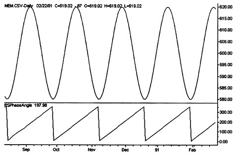
The last major characteristic of a primitive cycle is amplitude.  Amplitude is the power of a cycle and is independent of frequency and phase.  All three of these features make up a simple cycle.  Let’s now use them to plot a simple sine wave in Omega TradeStation, using the following formula: Value 1 = (Sine ((360 x Current Bar)/Period)*Amplitude) + Offset;

Using a period of 30, an amplitude of 20, and an offset of 600, these parameters produce the curve shown below, which looks a little like the S&P500 and shows how phase interacts with a simple sine wave.  Note that by using the TradeCycles phase indicator, tops occur at 180 degrees and bottoms occur at 0 degrees.

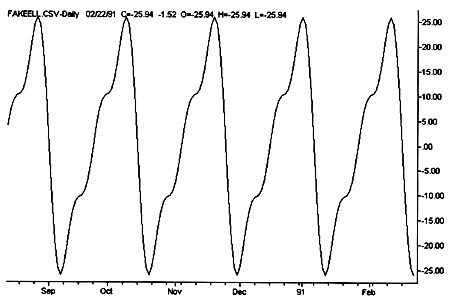
A simple sine wave is not very interesting, but by adding and subtracting harmonics we can produce a pattern that looks a little like an Elliot Wave.  Our formula is as follows:

This simple curve resembles an Elliott Wave pattern using a period of 30 and an amplitude of 20, as shown below.  This figure is an example of how chart patterns are actually made up of combinations of cycles.

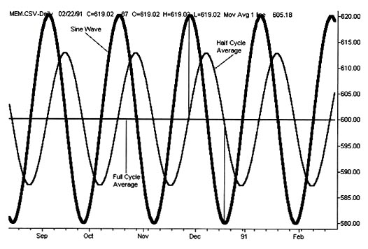
Let’s use our sine wave to test the relationship between cycles and a simple moving average.  We can start with a simple half-cycle moving average.  The lag in a half-cycle moving average is 90 degrees.  The figure below shows a sine wave curve, a half-period moving average, and a full-period moving average.  The full-period moving average is always zero because it has as many values below zero as above zero.

Let’s now build a simulated Elliott Wave with a period of 30 and an amplitude of 20.  If we trade the classic moving-average crossover system, we see that a 2-period and a 15-period moving average produce the best results (about 16.90 points per cycle).  This system bought just as our fake wave three took out our fake wave one to the upside, and it sold about one-third of the way down on the short side.  One the other hand, if we use the reverse rules and a 15-period and 30-period moving average, we then make over 53.00 points per cycle.  This system would buy at the bottom and sell about one-third before the top, or about at the point where wave five begins.  These results show that, in a pure cycle-based simulated market, the classic moving-average system would lose money.  In real life, moving-average systems only make money when a market moves into a trend mode, or because of shifting in cycles that causes changes in the phase of the moving averages to price.  We cannot predict these shifts in phase.  Unless a market trends, a system based on moving-average optimization cannot be expected to make money into the future.

Another classic indicator, the RSI, expresses the relative strength of the momentum in a given market.  Once again, we use our simulated Elliott Wave, based on a 3-day dominant cycle.  We have found that combining a 16-day RSI with the classic 30 and 70 levels produces good results, showing that RSI is really a cycle-based indicator.  Using a simulated market over 5 complete cycles, we produced over 59.00 points per cycle and the signals produced bought 1 day after the bottom sold and 3 days after the top.

Another classic system that actually works well in cycle mode and will continue to work in trend mode is a consecutive close system.  Channel breakout would also work, but you would want to use a 2-day high or low to maximize the profit based on our simulated Elliott Wave.  If you use a 1-day high, your trades would be whipsawed in waves two and four, as they would be in a real market, because the channel length is too short.

Now, let’s talk about using the MEM algorithm to trade cycles in the real world.  The MEM algorithm requires tuning of many technical parameters.  MESA  (Maximum Entropy Spectral Analysis) 1996 adjusts these parameters for you.  TradeCycles adjusts many of these parameters too, but it also lets you set the window and the number of poles.  Real financial data are noisy, so it is important to know the power of the dominant cycle.  We call the power, relative to the power of the rest of the spectra, the signal-to-noise ratio.  The higher the signal-to-noise ratio, the more reliable the cycle.  In TradeCycles, we calculate this ratio by determining the scaled amplitude of the dominant cycle and dividing it by the average strength of all frequencies.  The level of the signal-to-noise ratio tells us a lot about the markets.  Many times, the signal-to-noise ratio is lower when a market is in breakout mode.  When using MEM for cycle-based trading applications, the higher the signal-to-noise ratio the more reliable the trading results.  If we are using MEM for trend-based trading, then the signal-to-noise ration relationship is less clear.